Population Genetics
general approach
- evolution = changes in gene frequency
- gene frequency
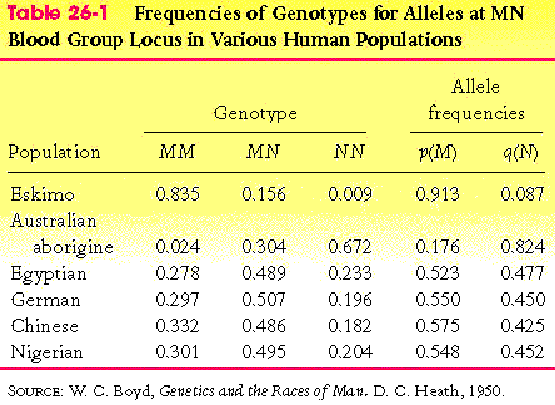
- see Table 26-1, p. 781

- make sure you understand the calculation of allele frequencies
from genotype frequencies
- genotype frequency
- see Table 26-1, p. 781
- population
- all individuals of a given species
in a local area that can mate with one another
- represented as a point in gene frequency
space
- often though of as a gene pool
- population variation
- genetic distance
- example from AIDS virus HIV
- heterozygosity
- measure of genetic variation
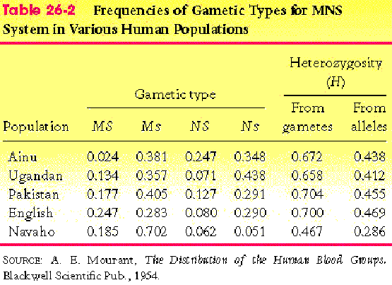
- two ways to calculate heterozygosity from
gametic types
- Table 26-2, p. 782

- MISTAKE IN TABLE 26-2: for English population the frequency of the Ns type should be 0.39 NOT 0.29
- use allele freqs. to calc. avg.
freq. heterozygotes at the two loci
- calc. gene frequency
- calc. expected heterozygotess
- average the freq. of expected heterozygotes
- from gamete freqs. directly
- use gamete freq. to calc. zygote freqs.
- include zygotes that are heterozygous for at
least one of the loci
Hardy-Weinberg law
- basic problem
- gene freqs --> genotype freqs
- genotype freqs --> gene freqs
(is easy)
- background
- don't worry about this stuff
- Castle in 1903
- denied by Yule 1908
- consider a dominant and recessive allele
A and a
- consider a cross between pure types: aa
X AA
- F1 cross:
- cross AA x aa ş>
Aa
- phenotype ratio 1:1 ş> 1:0
- F2 cross:
- cross Aa x Aa ş>
.25 AA .50 Aa .25 aa
- phenotype ratio 1:0 ş> 3
: 1
- Yule's conclusions
- ratio was the only stable ratio
for a dominant gene and would be reached from any initial frequency
- reasonable to suppose that the dominant
gene will take over and that ultimately a population's phenotypes
will be due to dominant genes with recessive genes existing as
rare mutants
- this implies that phenotypes would
exist not only because of their effects on fitness but also because
of Mendelian ratios (depending on dominance, etc)
- this has far reaching implications
for evolution
- instead Mendelism is more neutral
- assumptions
- random mating
- random union of gametes
- use Punnett square
- see calculations in text
- multiply gene freqs to get expected genotype
freqs
- no selection
- no migration
- no mutation
- infinite population size
- MN blood group
- background
- one of many redşblood cell antigenşantibody
systems
- two antigens: M and N
- single locus with two codominant alleles
- genotypes: MM, MN, NN
- phenotypes: M, MN, N
- observed and expected frequencies
- see Table 26-1
- general calculation
- genotype freqs in present generation
- AA: fAA
- Aa: fAa
- aa: faa
- may not be HW freqs
- gene freqs in present generation
from genotype frequencies
- p = fAA + 0.5 fAa
- q = 1 ş p = faa + 0.5 fAa
- genotype freqs in next generation
- AA: p2
- Aa: 2pq
- aa: q2
- these HW freqs are stable from then on
- gene freqs next generation
- pnext gen = p2 +
.5 * 2pq = p
- qnext gen = q2 +
.5 * 2pq = q
- gene freqs don't change
- overview of Hardy Weinberg Law
- HW law
- conclusions
- gene frequency equilibrium every
generation
- genotype frequency equilibrium attained
in a single generation
- forces
- mutation
- selection
- migration
- drift
- analogous to Newton's first law
- if no forces operate on an object, the
velocity and direction of motion is constant
- forces
- weak
- strong
- electromagnetic
- etc.
- analogous to Malthus' law
- if no forces operate on a population its
per capita growth rate is constant, r
- forces
- competition
- predation
- etc.
- provides foundation for model building
and explanations
- provides a null hypothesis
- consequences of HW law for rare alleles
- freq hets >> freq homo for
rare alleles: 2pq >> q2
- deleterious recessive genes
- cystic fibrosis
- gene
- autosomal recessive gene
- DNA sequence has open reading frame
- protein
- aa
- defective beta glucuronidase
- phenotype
- abnormal gladular secretions, death
before 20
- mucus builds up ş> suffocation
- q = freq of allele = .024
- 2pq = .047 = 1/21
- q2 = 1/1700
- each of us has about 10 such alleles
masked
- outcrossing functions to mask these
alleles
- testing for fit to HW
- observed versus expected frequencies
- describe 2 test
- numbers of observed and expected types
in each class
- degrees of freedom
- number of classes - number of items
calculated from data
- two loci
- don't worry about this stuff
- consider two loci: A, a
and B, b
- r = recombination rate
- p and q freqs of A and a
- r and s freqs of B and b
- gamete types:AB, Ab, aB, ab
- gamete freq:x1x2x3x4
- gene freqs
- p = x1 + x2, q =
x3 + x4
- r = x1 + x3, s =
x2 + x4
- linkage disequilibrium: D = x1x4
ş x2x3
- how to get from gene freqs to gamete
freqs?
- x1 = pr + D
- x2 = ps ş D
- x3 = qr ş D
- x4 = qs + D
- Dt+1
= (1 ş r ) Dt
- conclusions
- gene freqs constant
- gamete & zygotic freqs approach HW
with time
- D goes to zero with time at rate r
- linkage disequilibrium affects selection
evolutionary forces
- mutation
- migration
- selection
- fitness
- selection coefficient
- chance; genetic drift
mutation
- random with regard to fitness affect
- A ş> a at rate m,
p freq A, q freq a
- pt = ptş1(1
ş m)
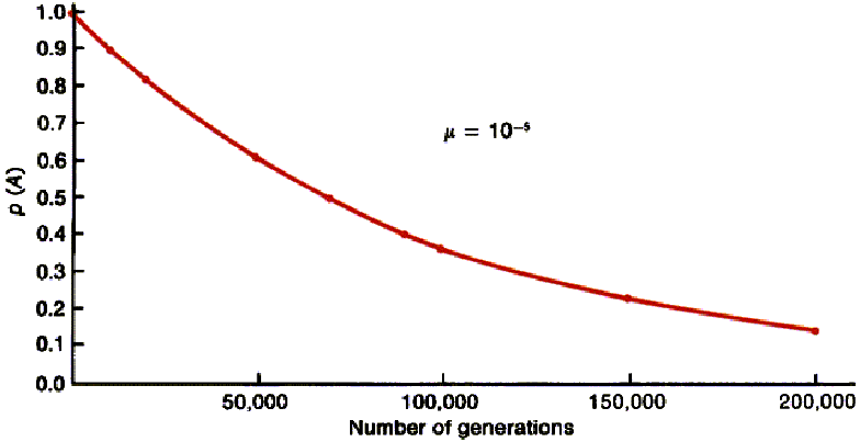
- for a single locus: m
= 10ş5
- weak force in changing gene freqs
- see Figure 26-9 in text

- although weak force in changing
gene frequencies mutation is still important in evolution
- recall Figure from lecture on mutation
and selection
- all variation ultimately stems from
mutation
natural selection
- propositions about nature (Darwin)
- variability
- heritability
- struggle to survive
- conclusion: natural selection must
occur
sickle cell anemia
- background
- we will use this as an example of
natural selection in human populations
- sickle cell anemia
- common in West and Central Africa
- gene freq reaches 16% in Africa
- up to 5% of the population dies
in infancy
- gene freq is about 5% for black
Americans
- geographic distribution correlated
with malaria
- why is the gene so widespread?
- hemoglobin molecule
- transport O2 in blood
- a
locus, ▀ locus
- tetramer = 2a
+ 2▀
- variation; alleles at b
locus
- A = wild type, in freq p
- S = sickle cell allele, in freq q
- C = recessive allele, in freq r
- "struggle to survive"
- data from West-African population
- relative and absolute fitness
- absolute fitness is expected numbers of offspring
- to obtain relative fitness divide absolute fitnesses by that of standard
- consider an example, letting Aa be the standard
| genotype | abs fitness
| rel fitness |
| AA | 9 | 0.9
|
| Aa | 10 | 1
|
| aa | 2 | 0.2
|
we will use relative fitness by letting genotype AS be the standard
| genotype | fitness
| condition |
| AA | 0.9 | malarial susceptible
|
| AS | 1.0 | malarial resistance
|
| SS | 0.2 | anemia
|
| AC | 0.9 | malarial susceptible
|
| SC | 0.7 | anemia
|
| CC | 1.3 | malarial resistance
|
questions
- S in high freqs of 0.10ş0.16, why?
- why doesn't C allele increase?
gene freq equations
- Dq =(pqwAS
+ q2wSS + qrwSC)/wavg
- q
- wavg = average fitness
- = W with over bar on p. 758
- equations on p. 758 are for two alleles
- Dq = qaS/wavg
- aS = pwAS
+ qwSS + rwSC - wavg
- aS = avg effect of the
S allele on fitness
- depends on fitness
- depends on gene and genotype frequencies
- sign of Dq
depends on sign of aS
- Dr = raC/wavg,
similarly
- aC = pwAC
+ qwSC + rwCC - wavg
application of gene freq equation
using aS
- pre-malaria African population
- malaria initially rare
- malaria was not important selective agent initially
- slash-and burn agriculture facilitates malaria
- African slash-and-burn agriculture began about
200 BC
- inc number of breeding places for mosquitos
- fixed for A (p=1, q=0, r=0)
- consider rare mutations from A to S or
C
- only heterozygote effect is important
- after malaria
- wavg = 0.9
- aS = (1)(1.0) - 0.9 =
.1 > 0
- conclusion: S allele increases rapidly
- aC = (1)(0.9) - 0.9 =
0
- conclusion: no selection for C
- homozygous effect not important for rare alleles
in outcrossing populations
- however, if inbreeding occurred aC > 0
- at equilibrium
- peq = 0.89, qeq
= 0.11, req = 0
- aS = 0
- aC = -0.03
- wavg = 0.91 <<
woptimal = wCC = 1.3
conclusion
- evolution not optimal
- evolution does not produce what
is best for the species
- natural selection has many components
natural selection has many components
- fitness
- intrinsic aspects
- environment
- mating system
- genetic system
- population structure
genetic structure in populations
- genetic variation
- how is it organized?
- within populations
- between individuals
- between populations
- human racial groups
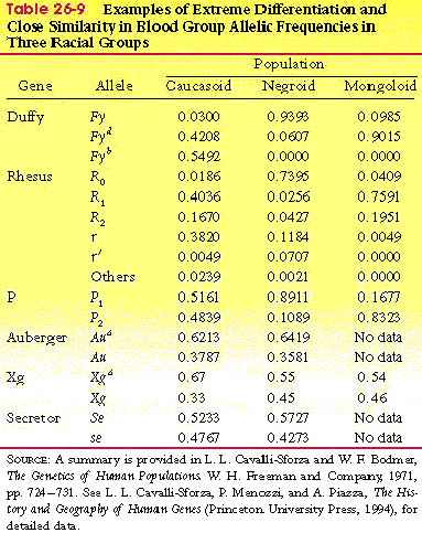
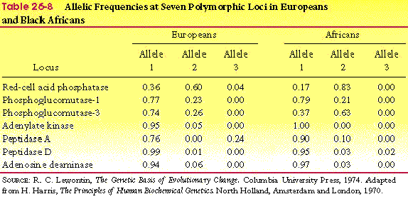
- some loci differ between races
- Table 26-9, p. 788

- Duffy
- still all races have all alleles
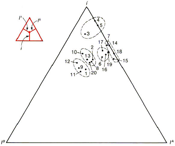
- genetic variation at most loci do not follow
racial boundaries
- Table 26-8, p. 787

- Fig 26-5, p. 788

- there is as much variation within races
as between
- there is no genetic basis for racial groups
- causes of population structure
- geographical subdivision
- lakes, streams, mountains
- resource distribution
- isolation by distance
- consequences of population structure
- non-random mating
- inbreeding
- inc. genetic relatedness
- dec. heterozygosity
- inc. homozygosity
- finite population structure
- genetic drift
- inbreeding
- mating between relatives
- identity by descent, ibd
- a kind of identity
- copies of the same DNA sequence in a common
ancestor
- example of ibd
- A*A x Aa
- here are their offspring: .25 A*A, .25 A*a, .25 AA, .25 Aa
- consider a sib mating: A*A x A*a
- here are the offspring of the sib mating: A*A*, .25 AA*, .25 A*a, .25 Aa
- the AA offspring contains identical alleles
- the A*A* offspring contains identical alleles that are also identical by descent, that is, identical
by being copies of the allele A* in the A*A grandparent
- inbreeding coefficient, F
- F = prob two alleles ibd
- alleles at same locus
- alleles picked from same individual
- effect of inbreeding on a single
population
- consider population with F
| AA | Aa |
aa |
| 1-F | p2 | 2pq
| q2 |
| F | p | |
q |
| (1-F)p2+pF |
(1-F)2pq | (1-F)q2+qF
|
| | |
|
dec heterozygosity
- HetF = (1-F) 2pq
increase in homosygosity
gene freqs unaffected by F
example: self fertilization
- see figure 26-12 of text p. 796
- note: gene frequencies stay the
same
effect of inbreeding in a subdivided
populations
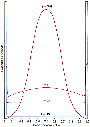
- big population made up of many smaller
populations
- Fig. 26-13, p. 797

- different populations fix (become homozygous)
for different alleles
- heterozygosity lost according to formula
on p. 796
- Ht = H0 (1
- 1/(2N))t
why 1/(2N)?
- consider diploid population of size
N: the chance of ibd is 1/(2N)
- for simplicity ignore the issue
of separate male and female sexes
- each individual produces k gametes
- random mating among these kN gametes
produced
- pick a gamete
- what is the chance another gamete
has a copy of the same allele ibd to the one just picked?
- there are (k/2)-1 other gametes that have alleles
ibd to the one just picked or approximately k/2 for k large
- so the chance of ibd is (k/2)/(kN) = 1/(2N)
coefficient of kinship, r
- measure of genetic relatedness
- used in calculations of inclusive fitness
- r = prob two alleles ibd
- alleles at same locus
- alleles picked from two different
individuals
- = F of a hypothetical offspring of the
two individuals
inbreeding depression
- lower fitness of inbred offspring
- fact of nature
- dominance hypothesis: masking of recessive
deleterious alleles
- overdominance: superior fitness of heterozygote
- application: evolution of sex
- sex
- recombination
- outcrossing
- outcrossing maintained by inbreeding
depression
genetic drift
- = changes in gene freq due to sampling
error
- sampling error is larger in small
populations
- consider a very small sample of
size 1
- if gene frequency is .5
- there is only a .50 chance of maintaining
that freq, that is of picking a heterozygote
- there is a .25 chance of the gene freq
being 1 in the sample (AA)
- there is a .25 chance of the gene freq
being 0 in the sample (aa)
- many mutations are neutral in their
effects on fitness and their evolution is determined by genetic
drift
|
